Zabbix in: exploratory data analysis rehearsal – Part 2

Abstract

In the previous blog post, we explored some of the basic statistical concepts to estimate KPIs for web application response time – average, median, and percentile. Additionally, we improved the nginx out-of-the-box template and showed some results in simple dashboards. Now it’s time to continue our work by analyzing some variances of the collected metrics and considering a certain period.

If you haven’t done so, please read the previous blog post to understand the context.

A little about basic statistics

In basic statistics, data distribution has at least four moments:

• Location estimate
• Variance
• Skewness
• Kurtosis

In the previous blog post, we introduced the first moment, knowing some estimates of our data distribution. It means that we have analyzed some values of our web application response time. It also reveals that the response time can have minimum and maximum values, averages, a value that can represent a central value of the distribution, and so on. Some metrics, such as averages, can be influenced by outliers. Others, such as 50^th percentile or median, cannot. Now we know something about the variance of those values, but it’s not enough. Let’s check the second moment of the data distribution – Variance.

Variance

We have some notion about the variance of the web application response time, meaning that it can have some asymmetry (in most cases). We also know that some KPIs must be considered – but which of them?

In exploratory data analysis, we can discover some key metrics, but in most cases we won’t use all of them, so we have to know each one’s relevance in order to choose properly which metric can represent the reality of our scenario.

There are some cases when some metrics must be added to other metrics so that they make sense. Otherwise, we can discard them – we must create and understand the context for all those metrics.

Let’s check some concepts of the variance:

• Variance
• Standard deviation
• Median absolute deviation (MAD)
• Amplitude
• IQR – Interquartile range

Amplitude

This concept is simple and so is its formula. It is the difference between the maximum and minimum value in a data distribution. In this case, we are talking about data distribution at the previous hour (,1h:now/h). We are interested in knowing the range of variation in response times in that period.

Let’s create a calculated item for the Amplitude metric in “Nginx by HTTP modified” template.

• trendmax(//net.tcp.service.perf[http,”{HOST.CONN}”,”{$NGINX.STUB_STATUS.PORT}”],1h:now/h)
• trendmin(//net.tcp.service.perf[http,”{HOST.CONN}”,”{$NGINX.STUB_STATUS.PORT}”],1h:now/h)

In other terms, it could be:

• max(/host/key)-min(/host/key)

However, we are analyzing a data distribution based on the previous hour, so:

• trendmax(/host/key,1h:now/h)-trendmin(/host/key,1h:now/h)

Modifying our dashboard, we’ll see something like this:

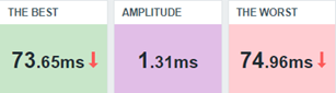
This resulting interpretation could be that between the worst and best response times, the variance is too small. It means that during that hour the response times had no significant differences.

However, amplitude itself is not enough to get some web application diagnosis at that moment. It’s necessary to combine this result with other results. Let’s see how to do it.

To complement, we can create some triggers based on it:

• Fire if the response time amplitude was bigger than 5 seconds at the previous hour. It means that the web application did not perform as expected considering the web application requests.
  • Expression = last(/Nginx by HTTP modified/amplitude.previous.hour)>5
  • Level = Information
• Fire if the response time amplitude reaches 5 seconds at least 3 consecutive times. It means that over the last 3 hours, there was too much unexpected variance among the web application response times.
  • Expression = min(/Nginx by HTTP modified/amplitude.previous.hour,#3)>5
  • Level = Warning

Remember, we are evaluating the previous hour and it makes no sense to generate this metric every single minute. Let’s create a custom interval period for it.

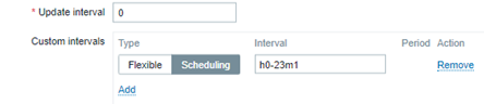
By doing so, we are avoiding flapping on the triggers in our environment.

IQR – Interquartile range

Consider these values below:

3, 5, 2, 1, 3, 3, 2, 6, 7, 8, 6, 7, 6

Open the shell environment. Create the file “vaules.txt” and insert each one, one per line. Now, read the file:

# cat values.txt

3
5
2
1
3
3
2
6
7
8
6
7
6

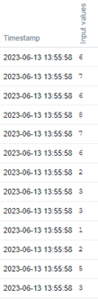
Now, send the value to Zabbix using Zabbix sender:

# for x in `cat values.txt`; do zabbix_sender -z 127.0.0.1 -s “Web server A” -k input.values -o $x; done

Look at the historical data using the Zabbix frontend.

Now, let’s create some Calculated items to the 75^th percentile and 25^th percentile.

• Key: iqr.test.75
  Formula: percentile(//input.values,#13,75)
  Type: Numeric (float)
• Key: iqr.test.25
  Formula: percentile(//input.values,#13,25)
  Type: Numeric (float)

If we apply the command “sort values.txt” on a Linux terminal, we’ll get the same values ordered by size. Let’s check:

# sort values.txt

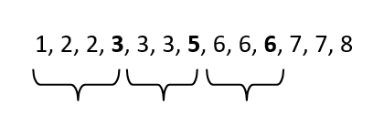
We’ll use the same concept here.

From the left to the right, go to the 25^th percentile. You will get the number 3.

Do it again, but this time go to the 50^th percentile. You will get the number 5.

And again, go to the 75^th percentile. You will get the number 6.

The IQR is the difference between the 75^th percentile (Q3) and the 25^th percentile (Q1). So, we are excluding the outliers (the smallest values on the left and the biggest values on the right).

To calculate the IQR, you can create the following calculate item:

• key: iqr.test
  Formula: last(//iqr.test.75)-last(//iqr.test.25)

Now, we’ll apply this concept in web application response time.

The calculated Item for the 75^th percentile:

key: percentile.75.response.time.previous.hour
Formula: percentile(//net.tcp.service.perf[http,”{HOST.CONN}”,”{$NGINX.STUB_STATUS.PORT}”],1h:now/h,75)

The calculated item for the 25th percentile:

key: percentile.25.response.time.previous.hour
Formula: percentile(//net.tcp.service.perf[http,”{HOST.CONN}”,”{$NGINX.STUB_STATUS.PORT}”],1h:now/h,25)

The calculated item for the IQR:

key: iqr.response.time.previous.hour
Formula: last(//percentile.75.response.time.previous.hour)-last(//percentile.25.response.time.previous.hour)

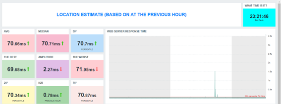
Keep the monitoring schedule at the first minute for each hour, to avoid repetition (very important) and adjust the dashboard.

Considering the worst web response time and the best web response time at the previous hour, the AMPLITUDE returns a big value in comparison to the IQR, It happens because the outliers were discarded in IQR calculation. So, just as the mean is a location estimate that is influenced by outliers and the median is not, so are the RANGE and IQR. The IQR is a robust indicator and allows us to know the difference between the web response time variance in a central position.

P.S. We are considering only the previous hour, but you can apply the IQR concept to an entire period, such as the previous day, week, or month using the correct time shift notation. You can use it to compare the web application response time variance between the periods you wish to observe and then get some insights about the web application behavior at different times and in different situations.

Variance

The variance is a way to calculate the dispersion of data, considering its average. In Zabbix, calculating the variance is simple, since there is a specific formula for it via a calculated item.

The formula is as follows:

• Key: varpop.response.time.previous.hour
  Formula: varpop(//net.tcp.service.perf[http,”{HOST.CONN}”,”{$NGINX.STUB_STATUS.PORT}”],1h:now/h)

In this case, the formula returns the dispersion of data, but there is a characteristic – at some point, the data is squared and the data scale changes.

Let’s check the steps for calculating the variance of the data:

1) Calculate the mean;
2) Subtract the mean of each value;
3) Square each subtraction result;
4) Perform the sum of all squares;
5) Divide the result of the sum by the total observations.

At the third step, we have the scale change. This new data can be used for other calculations in the future.

Standard Deviation

The root square of the variance.

Calculating the root square of the variance, the data can come back to its original scale!

There are at least two ways to do it:

1. Using the root square key and formula in Zabbix:
   1. Key: varpop.previous.hour
   2. Formula: sqrt(last(//varpop.response.time.previous.hour))
2. Using the standard deviation key and formula in Zabbix:
   1. Key:previous.hour
   2. Formula: stddevpop(//host,key,1h:now/h) # an example for the previous hour

A simple way to understand the standard deviation concept is by seeing it as a way of knowing how “far” values are from the average. So, applying the specific formula, we’ll get that indicator.

Take a look at the following image:

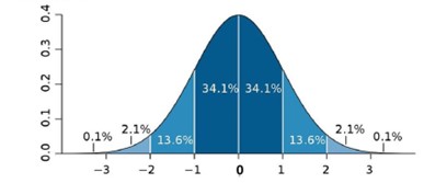
The image above is a common image that can be found on the internet, and it can help us understand some results. The standard deviation value must be near “zero”, otherwise, we’ll have serious deviations.

Let’s check the following calculated item:

• stddevpop(//net.tcp.service.perf[http,”{HOST.CONN}”,”{$NGINX.STUB_STATUS.PORT}”],1h:now/h)

We are calculating the standard deviation based on the collected values at the previous hour. Let’s check the test item in the frontend:

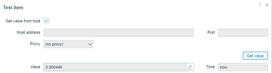
The test returned some value less than 1, at about 0.000446. If this value is less than 1, we don’t have a complete deviation and it means that the collected values at the previous hour are near the average.

For web application response time it can represent good behavior with no significant variances. Of course, other indicators must be checked for a complete and reliable diagnosis.

Important notes about standard deviation:

• It is sensitive to outliers
• It can be calculated based on the population of a data distribution or based on its sample.
  • Use this formula: stddevsamp. In this case, it can return a different value from the previous one.

Median Absolute Deviation (MAD)

While the standard deviation is a simple way to understand if the data of a distribution are far from its mean, MAD helps us understand if these values are far from its median. Therefore, MAD can be considered a robust estimate, because it is not sensitive to outliers.

Warning: If you need to identify outliers or consider them in your analysis, the MAD function is not recommended, because it ignores them.

Let’s check our dashboard and compare different deviation calculations for the same data distribution:

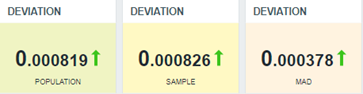
Note that the last one is based on the MAD function, and it is less than the other items because it is not considering outliers.

In this particular case, the web application is stable and its response times are near to the mean or median (considering the MAD algorithm).

Exploratory Dashboard

Partial conclusion

In this post, we have introduced the data distribution moments, presenting the variability or variance concept and learning some techniques to meet some KPIs or indicators.

What have we learned? The response time for a web application can be different from the previous one, so the knowledge of the variance can help us understand the application behaviors using some extraordinary data. Then we can make judgments about an application’s performance.

Of course, it was a didactic example for some data distribution, and the location estimate and variance concepts can be applied to other data exploratory analysis considering a long period. In those cases, it is very important to consider using trends instead of historical data.

Our goal is to bring to light some extraordinary data and insights that will allow us to better understand our application.

In the next posts, we’ll talk about Skewness and Kurtosis, the third and fourth moments for data distribution, respectively.

About Paulo R. Deolindo Jr.

Zabbix Trainer at Unirede

View all posts by Paulo R. Deolindo Jr.