Table of Contents
Abstract
This will be the last blog post of the “Zabbix in… exploratory data analysis rehearsal” series. To continue our initial proposal, we’ll close the third and fourth data distribution moments concept. This time, we’ll talk about Skewness and Kurtosis.
Remember the first and second articles of the series to be aware of what we are discussing here.
The four moments for a data distribution
While the first moment helps us with the location estimate for some data distribution, the second moment works with its variance. The third moment, called asymmetry, allows us to understand the value trends and the degree of the asymmetry. The fourth moment is called kurtosis and is about the probability of the peak’s existence (outliers).
These four moments are not the final study about the data distribution. There is so much to learn and apply to data science when considering statistical concepts, but for now we must finish the initial proposal and bring forward some insights for decision makers.
Let’s get started!
Asymmetry
Based on our web application scenario, we can see a certain asymmetry in response time in most cases. This is normal and expected – so far, no problems. But it is also true that some symmetry is also possible in certain cases. Again, no problems here.
So, where is the problem? When does it happen?
Sometimes, the web application response time can be too different from the previous one, and we have no control over it. In these cases, the outliers must be found, and the correct interpretation must be applied. At that point, we must consider anomalies in the environment. Sometimes, the outliers are just a deviation. In all cases, we must pay attention and monitor the metrics that can make the difference.
Speaking of asymmetry – why is this topic so special? One of the possible answers is that we need to understand the degree of the asymmetry – whether it is high or moderated and whether the values were in most cases smaller than or bigger than the mean or median. In other words, what does the asymmetry say about the web application performance?
Let’s check some implementations.
The key skewness
From version 6.0, Zabbix introduced the item key skewness.
For example, it can be used like this:
skewness(/host/key,1h) # the skewness for the last hour until now
Now, let’s see how this formula could be applied to our scenario:
skewness(//net.tcp.service.perf[http,”{HOST.CONN}”,”{$NGINX.STUB_STATUS.PORT}”],1h:now/h)
Using skewness and time shift “1h:now/h”, we are looking for some web application response time asymmetry at the previous hour.
The asymmetry can be negative (left skew), zero, positive (right skew) or undefined.

Definition: a left-skewed distribution is longer on the left side of its peak than on its right. In other words, a left-skewed distribution has a long tail on its left side.
Considering a left skew, it is possible to state that at the previous hour, the web application had more higher values than smaller values. This means that our web application does not perform as well as it should.

Look at the graph above. You can see some bars on the left side of the mean and other bars on the right side of the mean, with the same size as a mirror. We can consider this a normal distribution for web application response time, but it does not mean that the response times were good or bad – it only means that they had some balance and suggests more investigation.

Definition: a right-skewed distribution is longer on the right side of its peak than on its left. In other words, a right-skewed distribution has a long tail on its right side.
Considering a right skew, it is possible to state that at the previous hour, the web application had more smaller values than higher values. This means our web application performs as expected.
Value Map for Skewness
You must create in your template the following value map:
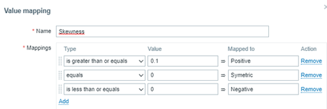
If you wish, the value map can also be as below:
“is greater than or equals” 0.1 à Mais tempos bons, se comparados à média
“equals” 0 à Tempos de resposta simétricos ou bem distribuídos em bons e ruins
“is less than or equals” 0 à Mais tempos ruins, se comparados à média
Pearson Skewness Coefficient
The Pearson’s Coefficient is a very interesting indicator. Considering some skewness for a data distribution, it tells us if the asymmetry is strong or only moderate.
We can create a calculated item for the Pearson’s Coefficient:
(3*(avg-median))/stddevpop
In Zabbix, we need:
- One item for the response time average considering the previous hour:
- Key: resp.time.previous.hour
- Formula: trendavg(//net.tcp.service.perf[http,”{HOST.CONN}”,”{$NGINX.STUB_STATUS.PORT}”],1h:now/h)
- One item for calculating the median (for percentile, see the previous blog post):
- Key: response.time.previous.hour
- Formula: (last(//p51.previous.hour)+last(//p50.previous.hour))/2
- One item for the standard deviation calculation:
- Key:
- Formula: response.time.previous.hour stddevpop(//net.tcp.service.perf[http,”{HOST.CONN}”,”{$NGINX.STUB_STATUS.PORT}”],1h:now/h)
- Key:
- Key: response.time.previous.hour
- Key: resp.time.previous.hour
Finally, a calculated item for a Pearson’s Coefficient:
- Key: coefficient.requests.previous.hour
- Formula:
((last(//trendavg.requests.per.minute)-
last(//median.access.previous.hour))*3)
/
last(//stddevpop.requests.previous.hour)
- Formula:
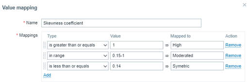
To finish the exercise, create a value map:
Curtose
Kurtosis is the fourth data distribution and can indicate if the values are prone to peaks.
In Zabbix, you can implement or calculate kurtosis with other calculated items:
kurtosis(/host/key,1h)
Um valor negativo de curtose nos diz que a distribuição não está propensa ou produziu poucos outliers. Já um valor positivo de curtose nos diz que a distribuição está propensa ou produziu muitos outliers. Tudo gira em torno da média da distribuição de dados. Já um valor neutro, ou zero, nos diz que a distribuição é considerada simétrica.
Para nosso cenário web, temos:
kurtosis(//net.tcp.service.perf[http,”{HOST.CONN}”,”{$NGINX.STUB_STATUS.PORT}”],1h:now/h)
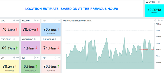
Explanatory Dashboard
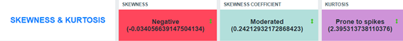
Considering the image above, the data distribution for the web application response time at the previous hour has a left skew. This suggests that, when considering the response time mean at the previous hour, there were more higher values than smallest values. That’s sad – our web application performed poorly. Why?
However, because the skewness was moderated (considering the Pearson’s Coefficient), it means that the response time values were not so different from the others at the same hour.
As for kurtosis, we can say that the data distribution is prone to peaks because we have positive kurtosis. In basic statistics, the values are near the mean and there is a high probability of producing outliers.
This is a point to pay attention to if you are looking at a critical service.
Looking at other metrics
To check and validate our interpretation, let’s visualize the collected values on a simple Zabbix graph, using a graph widget.
Please consider using the following “time period” configuration:
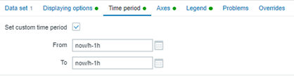
The graph will show only the data collected at the previous hour – in this case, from 11:00 to 11:59.
The graph in Zabbix allows us to visualize the 50th percentile as well. We do not display the mean on the graph because it wouldn’t be well represented visually as it was collected only once, thus lacking an interesting visual trend line like the 50th percentile. However, notice that the mean and the 50th percentile values are very close, which will give us an idea of the data distribution around this measure.
Partial Conclusion
Skewness and Kurtosis, respectively, are the third and fourth moments of a data distribution. They help us understand the environment’s behavior and allow us to gain insight into a lot of things (in this case, we simply applied these concepts to IT infrastructure monitoring and focused on our web application to analyze its performance).
In most cases, the asymmetry will exist – it’s normal and expected. However, knowing some properties of the skewness can help us understand the response times, indicating good or poor performance. The skewness coefficient allows us to know if the asymmetry was strong or just moderated. Meanwhile, kurtosis helps us to understand if the data distribution produced some peaks considering an observation period or whether it is prone to produce peaks. We can then create some triggers for that and avoid some undesirable behaviors in the future, based on our data distribution observation. This is applied data science at its best.
Conclusion
Data science can be easily applied to (and bring up insights about) Zabbix and its Aggregate functions. It’s true that there are some special functions such as skewness, kurtosis, stddevpop, stddevsamp, mad, and so on, but there are old functions to help us too, such as percentile, forecast, timeleft, etc. All these functions must be used in calculated item formulas.
One of the interesting advantages of using Zabbix in data science and performing an exploratory data analysis is the fact that Zabbix can monitor everything. This means that the database already exists with the relevant date to analyze, in real time.
In the blog posts in this series, we took as a basis some data referring to the previous hour, the previous day, and so on, but we did nothing regarding the current hour. If we applied the concepts studied in real time data, we would have other “live” results, including support for decision-making. This is because we will not only study historical data, but instead will have the opportunity to change the course of events.
Zabbix is improving dashboards significantly. From Zabbix 6.4, we have many new out-of-the-box widgets and the possibility to create our own. However, there is a concern – Zabbix administrators sometimes show unnecessary data in dashboards, which can cloud the decision-making process. Zabbix administrators, in general, might want to learn storytelling techniques to rectify this situation. Maybe in a perfect world!
I hope you have enjoyed this blog post series.
Keep studying!